Disk Imaging

Astro 497, Week 12, Friday

Acknowledgement to Prof. Ian Czekala's Astro 542 and Astro 589.

Types of Disks

Protostellar
- Circumstellar
- Circumbinary
Protoplanetary
- Gas/Primary
- Dusk/Debris

Protostellar cores collapsing to form stars

When the core becomes gravitationally unstable, it will begin to collapse.

The free-fall timescale is

$$\tau = \sqrt{\frac{3 \pi}{32 G \rho}}$$

Optically thick, so can't see into what's happening at this phase.

let
 	G = 6.6743e-8 # cm^3 g^-1 s
    ρ_sol  = 1.41
    sec_in_day = 24*60*60
    days_in_year = 365.2425
    τ = sqrt(3π/(32*G*ρ_sol)) / sec_in_day
    r = 10.0.^(-2:0.25:2)
    r_sol = 0.005
    scalefontsizes()
    scalefontsizes(1.5)
    plot(r, τ.*(r./r_sol).^3 ./days_in_year, 
        linewidth=4,
        xscale=:log10, yscale=:log10, legend=:none)
    xlabel!("r (AU)")
    ylabel!("τ (Years)")
end

Protostar classes

Protostellar systems (protostars and their disks) are conventionally divided into four different classes based on the overall shape of their infrared spectrum, characterized by their spectral index

$$\alpha \equiv \frac{d \log(\lambda F_\lambda)}{d \log \lambda}.$$

i.e.,

$$\nu F_\nu \propto \nu^{-\alpha}.$$

Observationally, this is usually calculated using observations done at 2.2 microns (K-band) and 10 microns (N-band), which are observable from the ground.

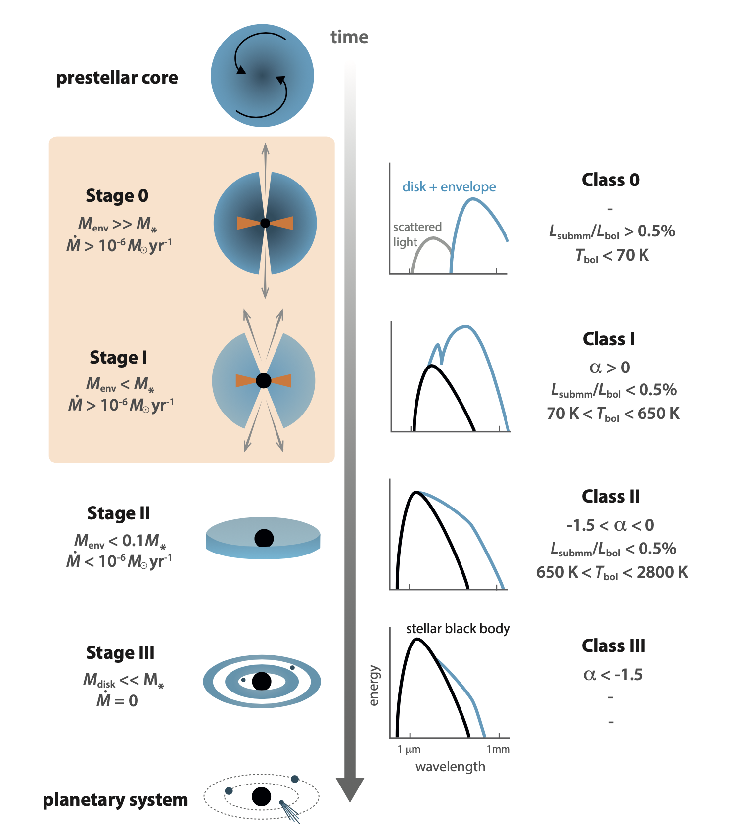
Schematic overview of the different stages of low-mass star formation (left) and the observational classification based on the spectral energy distribution (right). Credit: Merel van’t Hoff, Ph.D. thesis.

Planets can be recognized by their sculpting of Stage III protoplanetary disks.

Question:

How does the type of star affect the characteristics of the protoplanetary disk?

More massive stars have more massive protoplanetary disks (initially).
Eventually, the disk disperses
Age of star/disk is most important parameter.

Question:

Are certain disk classes more common than others?

Every star passes through each stage
Observed occurence rate tells us about how long a star spends in each stage.
Entire process
Until large mid-IR surveys, Stage 0 were rare because most emission in mid-IR
Stage I disks are rare because they collapse quickly
Stage II disks are relatively common.
Stage III stage can last millions of years, but they are are rarely detected because they are hard to detect disks when they have low mass mass
Transitional disks (with both gas and dust) are particularly valuable, but also rare because gas is rapidly dispersing as dust emerges.

question_box(md"Is there a limit to how long a protoplanetary disc can last, and what might happen to it after its lifetime has come to an end?")

Question:

Is there a limit to how long a protoplanetary disc can last, and what might happen to it after its lifetime has come to an end?

–- Credit: Mamajek 2009 Lincense: CC BY-SA 3.0

question_box(md"When measuring a disk mass, are we able to tell how wide the disk is from out perspective or are we assuming the volume to be a chosen value?")

Question:

When measuring a disk mass, are we able to tell how wide the disk is from out perspective or are we assuming the volume to be a chosen value?

Infrared Excesses

Most systems are so far away that don't resolve disks
Measuring excess emission in IR (relative to model for star) provides evidence for disks and estimates of their mass.
The closest stars with infrared excesses make great targets for disk imaging.

Disk observations as a function of wavelength

Optical (and some NIR) observations

Optically thick:
- Disk blocks starlight/other parts of disk
- Requires detailed modeling
Optically thin:
- See light scattered by grains
Atmosphere makes detecting faint disks close to star difficult
Hubble Space Telescope best source of good disk images in optical

IR observations

See thermal emission (plus molecular transitions)
Often measure IR excess, but too far away to resolve disk.
Lower spatial resolution for given size observatory due to diffraction limit
Ground-based observatories have larger aperture than HST
Adaptive optics starts to become effective in near-IR
Great images of nearby diks from Ground-based observatories with sophisticated AO systems
Disks are particularly challenging due to high contrast ratio.

Sub-mm & Radio observations

See thermal emission from dust
See molecular transitions (especially rotation)
Hyperfine splitting (e.g., 21 cm)
Single disk observations have low resolution due to long wavelength
Interferometry becomes practical in sub-mm and allows for even better resolution

ALMA

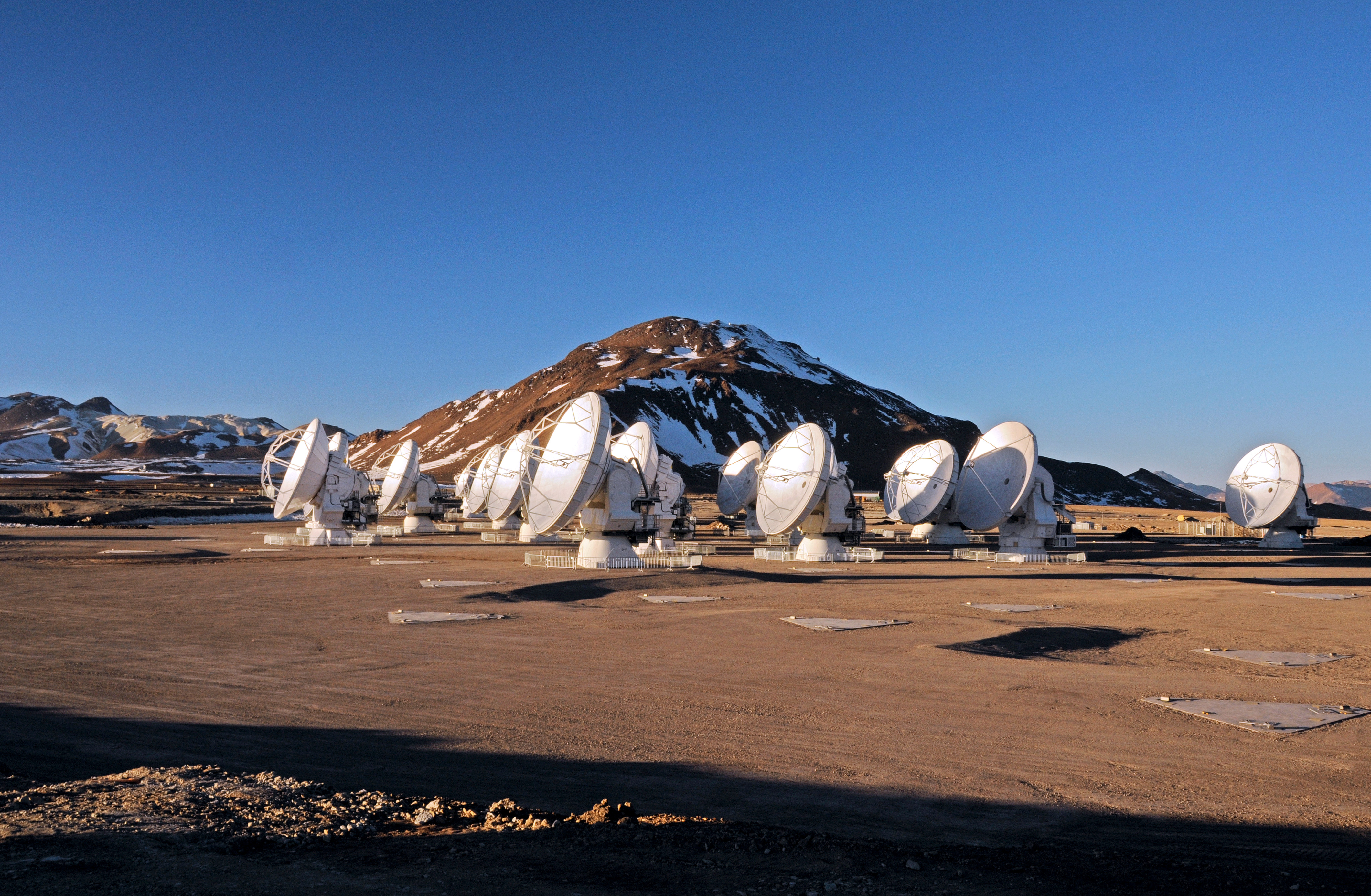
The Atacama Large (Sub)millimeter Array, an interferometric array of 66 antennas operating at sub-millimeter wavelengths. The largest antennas in the array are only 12m in diameter, yet through interferometry, the array is able to obtain far higher spatial resolution than the largest single-dish antennas. Credit: NRAO/ESO/NAOJ/JAO

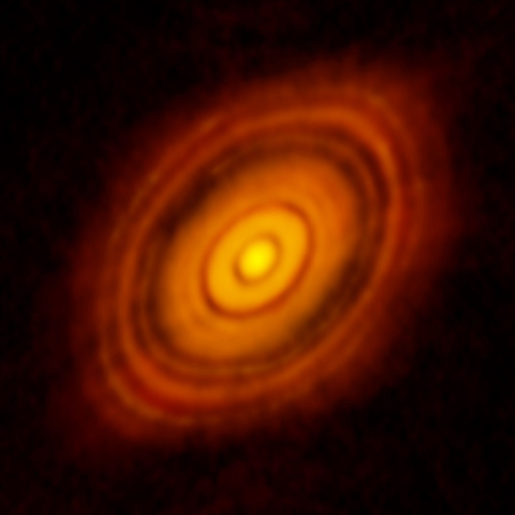
The protoplanetary disk around HL Tau, imaged using the Atacama Large Millimeter Array. Credit: ALMA(ESO/NAOJ/NRAO); C. Brogan, B. Saxton (NRAO/AUI/NSF)

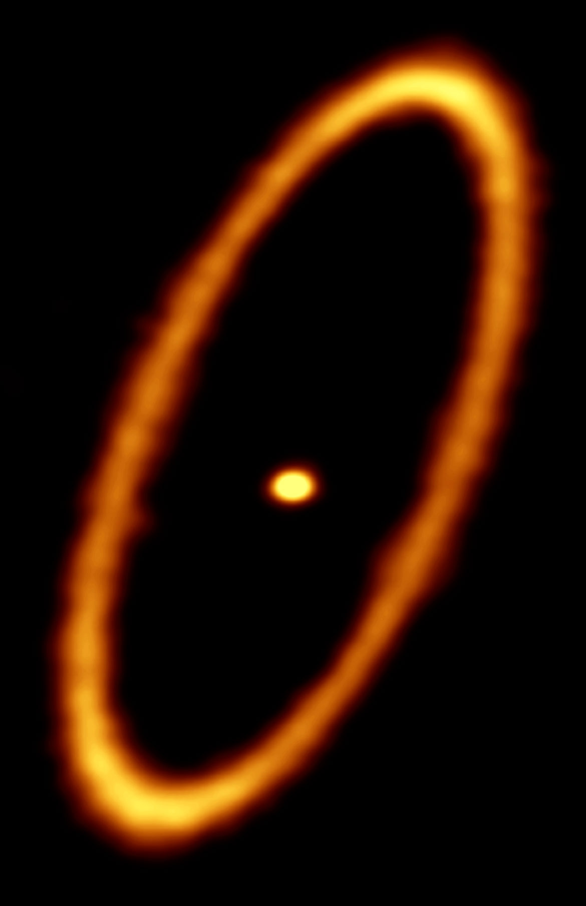
–- Credit: ALMA (ESO/NAOJ/NRAO); M. MacGregor

Key Questions about a Disk:

Optically thin or thick?
How old is disk?
What process is depleting disk?
Is disk being replenished?

Key Questions about an observation?

What wavelength?
What size particles are we seeing?

Reading Questions

question_box(md"How is the mass outflow of a protoplanetary disk measured?")

Question:

How is the mass outflow of a protoplanetary disk measured?

Measuring Mass from Optically Thin Disk

Emission proportional to surface area of scatterers
Estimate equilibrium temperature based on host star temperature & distance
Surface area to mass ratio depense on size distribution
Model size distribution as collisional cascade
Infer mass of scatterers via mass absorption coefficient ($\kappa$)
Omits mass in gas (& much smaller grains)

Setup

begin
    using PlutoUI, PlutoTeachingTools
    using Plots
end

Built with Julia 1.8.2 and

Plots 1.35.8
PlutoTeachingTools 0.2.5
PlutoUI 0.7.48

To run this tutorial locally, download this file and open it with Pluto.jl.