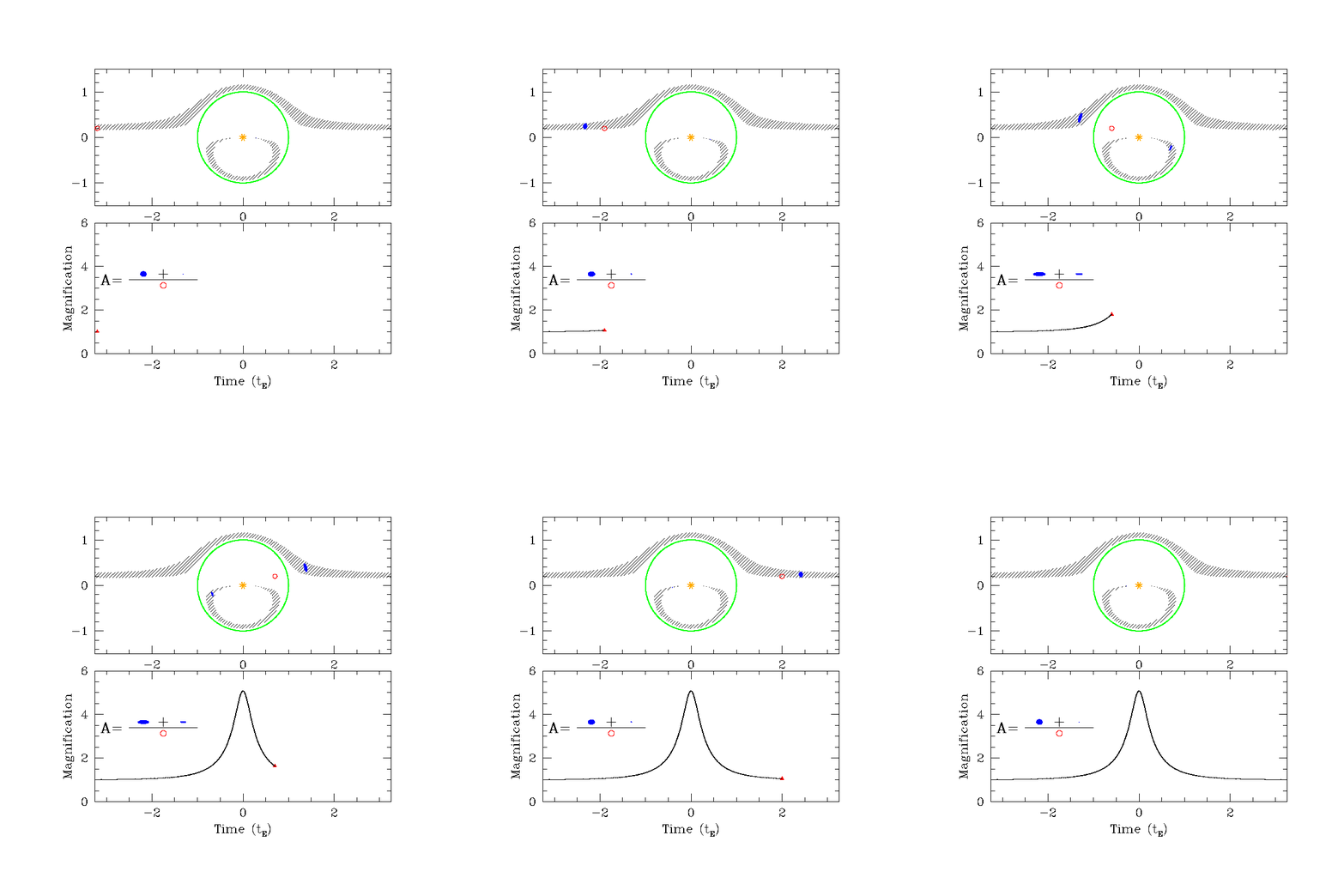
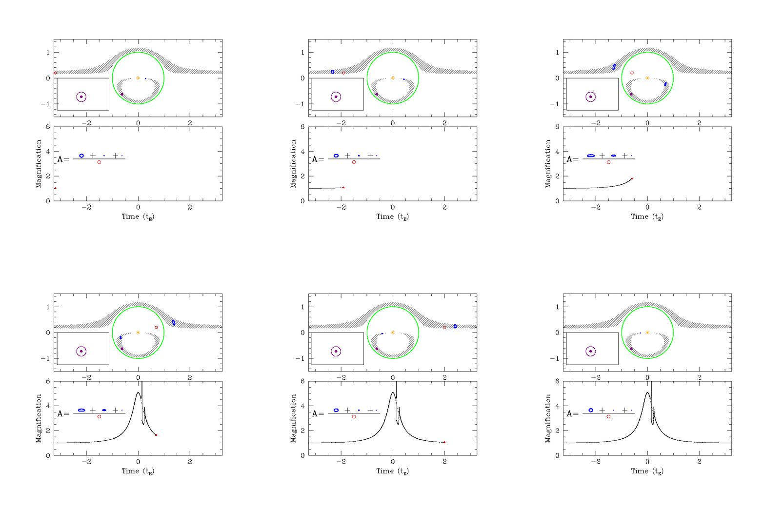
Microlensing

Astro 497, Week 11, Friday

Logistics

Please read Feedback on Project Checkpoint 1
Let me know if you have questions

TableOfContents()

Einstein radius

$$\theta_E = \sqrt{\frac{2R_{Sch}}{D_{rel}}} = \frac{2\sqrt{GM_l}}{c}$$

$G$: Gravitational constant
$M_l$: Mass of lens
$c$: speed of light
$D_l$: Distance to lens
$D_s$: Distance to source
$D_{rel}$: Relative distance. $1/D_{rel} = 1/D_l - 1/D_s$

Physical separation of Einstein ring at distance of lens

$$r_E = \theta_E D_l \simeq 2.2 \mathrm{AU} \left(\frac{M_l}{0.3 M_\odot}\right)^{1/2} \left(\frac{D_s}{8 \mathrm{kpc}}\right)^{1/2} \left(\frac{x(1-x)}{0.25}\right)^{1/2}$$

$$x\equiv D_l/D_s$$

Magnification ($A$)

Can be 10%, 100% or even 1000%!
$A>1.34$ if $u\le 1$
Even if $r_E$ is very small

Single Lens

–- Credit: S. Gaudi

Timescale for Microlensing Events

$$t_E = \theta_E / \mu_{\mathrm{rel}}$$

$\mu_{\mathrm{rel}}$: proper motion of source relative to the lens
Often $\sim$months for low-mass star lens events towards galactic bulge

Lens with Planet

–- Credit: S. Gaudi

Frequency of microlensing events

$\mathcal{O}(10^{-6})$ events per star per year
Towards buldge $\sim~10^7$ stars per deg² to I$\sim~20$
$\sim~10$ events per square degree monitored

question_box(md"Have any known microlensing events for an exoplanet been caused by a black hole rather than a background star?")

Question:

Have any known microlensing events for an exoplanet been caused by a black hole rather than a background star?

if D_l>=D_s
  warning_box(md"Distance to lens must be less than distance to source.")
end

plot(plt_sky_obs,plt_lc_star_obs, plt_sky_theory, plt_lc_star_theory, layout=grid(2,2), size=(800,800) )

Lens Star Properties: D_l: kpc M_l: M_⊙

Source Star Properties: D_s: kpc R_s: R_⊙

Relative Position/Velocity: b₀ (star): AU v_rel,sky: km/s

Observer Plot Limits: Distance: AU Time: d Magnification:

Add Planet: M_l,pl: M_⊕ x_pl: AU y_pl: AU

r_E: 2.2 AU r_E,pl: 0.022 AU t_E,⋆: 127.0 d t_E,pl: 1.27 d r_pl: 1.41 AU

Planet Hunting Regimes

Weak magnification regime

$A\le~10$ or $u_0\ge0.1$
$\theta_{E,p} = \sqrt{\frac{m_pl}{M_l}}$
Probability of significant additional magnification by planet: $\sim A(t_{0,p}) \theta_{E,p} / \theta_E$
Sensitivity to planets:
- Peaks when projected planet-star separation is comparable to $r_E$
- Falls rapidly for planets inside $r_E$, more slowly for planets beyond $r_E$
Detection is challenging primarily because planetary events have short durations and could fall in gaps between observations.
Relatively easy to model
$t_E$ provides information about lens mass, distance and relative proper motion
$A_{pl}$ and time of planetary event constrain projected separation (in units of $r_E$)

Strong magnification regime

$u\le 0.01$ or $A_\max \ge 100$
Events with maximum magnification $A_\max$ are small fraction of events ($\sim1/A_\max$)
Sensitive to planets with projected separation $\simeq r_E$ regardless of azimuthal angle
$\sim~1$ day of high sensitivity
Time of peak sensitivity can be predicted with hours to days of lead time
Modeling is complex and computationally expensive (And not included in figure above.)
Can help resolve some degeneracies in planet mass and separation
Often still two qualitatively different solutions (corresponding to very close/very wide solutions)

Higher-order effects

Blending with background stars
Finite source size
Parallax effects
Orbital motion of lens system
Binary sources

Microlensing Pros

Sensitive to relatively low-mass planets at intermediate distances
Even low-mass planets cause substantial increases in observed flux (for a brief time)
Potential to link occurence rates measured by transit/Doppler surveys to occurence direct imaging surveys
Opportunity for small telescopes to make valuable contributions
Potential to detect sub-Earth-mass planets
Potential to detect free-floating planets
Several degeneracies in basic scenario can be resolved by combining multiple observatories spread across the solar system.

Microlensing Cons

Don't get to pick to apply microlensing to a system
Majority of microlensing events provide limited information about planets
Planetary systems detected are faint & far away
Unlikely to get a second chance to study a given system
Need intense monitoring to detect brief magnification events from low-mass planets
Low sensitivity to planets significantly closer than Eienstein radius
Often significant degeneracies in measured parameters
Difficult to distinguish planets on wide orbits from free-floating planets
Limited observatories beyond Earth orbit to help resolve degeneracies

Programming Collaborations

Setup/Helper Code

ChooseDisplayMode()

Full Width Mode Present Mode

begin
    using PlutoUI, PlutoTeachingTools
    using Plots, Plots.Measures, ColorSchemes, LaTeXStrings
end

Microlensing Plots

begin  
    # Computer intermediate results for stellar lens
    local x = D_l/D_s
    r_e = 2.2*sqrt( (M_l_star/0.3) * D_s/8 * x*(1-x)/0.25 ) # AU
    u₀_star = b₀_star  / r_e  
    v_lens_au_per_day = v_lens_km_per_sec / AU_to_km * sec_to_day
    tₑ_star = r_e/v_lens_au_per_day	
    min_u_star = (Rsol_at_kpc * R_s / D_s) * (D_l*1000*parsec_to_AU) / r_e # very approximate
end;

begin
    # Computer intermediate results for planet lens
    M_l_pl = M_l_pl_earth * 3e-6
    r_e_pl = r_e * sqrt( M_l_pl/M_l_star ) # AU
    tₑ_pl = tₑ_star * sqrt(M_l_pl/M_l_star)
    r_pl = sqrt(x_pl^2+y_pl^2)
    u₀_pl = (y_pl - b₀_star)/r_e_pl
    t₀_pl = x_pl/v_lens_au_per_day # / v_rel
    min_u_pl = (Rsol_at_kpc * R_s / D_s) * (D_l*1000*parsec_to_AU) / r_e_pl # very approximate
end;

begin
    local plt_lim = sky_plt_lim
    plt_sky_obs = plot(xlabel=L"x \; (\mathrm{AU})", ylabel=L"y \; (\mathrm{AU})", 
        size=(600,600), frame=:box, legend=:none, 
        left_margin=2.5*Plots.mm, bottom_margin=2*Plots.mm)
    xlims!(plt_sky_obs,-plt_lim,plt_lim)
    ylims!(plt_sky_obs,-plt_lim,plt_lim)
    plot_circle!(plt_sky_obs,r_e)
    plot!(plt_sky_obs, [-plt_lim,plt_lim],[b₀_star, b₀_star], linewidth=4, linestyle=:dot )
    if incl_planet 
        plot_circle!(plt_sky_obs,r_e*sqrt(M_l_pl/M_l_star), x=x_pl, y=y_pl, linecolor=3, linestyle=:dot)
        scatter!(plt_sky_obs, [x_pl], [y_pl], markersize=4, markerstrokewidth=0, markercolor=3)
    end
    plt_sky_obs
end;

begin
    local plt_lim = 2
    plt_sky_theory = plot(xlabel=L"x \; (r_E)", ylabel=L"y \; (r_E)", 
        size=(600,600), frame=:box, legend=:none, 
        left_margin=2.5*Plots.mm, bottom_margin=2*Plots.mm)
    xlims!(plt_sky_theory,-plt_lim,plt_lim)
    ylims!(plt_sky_theory,-plt_lim,plt_lim)
    plot_circle!(plt_sky_theory,1)
    plot!(plt_sky_theory, [-plt_lim,plt_lim],[u₀_star, u₀_star], linewidth=4, linestyle=:dot )
    if incl_planet 
        plot_circle!(plt_sky_theory,sqrt(M_l_pl/M_l_star), x=x_pl/r_e, y=y_pl/r_e, linecolor=3, linestyle=:dot)
        scatter!(plt_sky_theory, [x_pl/r_e], [y_pl/r_e], markersize=4, markerstrokewidth=0, markercolor=3)
    end
    plt_sky_theory
end;

begin
    local plt_lim = lc_plt_lim
    plt_lc_star_obs = plot(xlabel = "Time (d)", ylabel="Magnification", 
        legend=:none)
    ylims!(0.9,lc_mag_lim)
    local t = range(-plt_lim,stop=plt_lim, step=0.02*tₑ_star)
    if incl_planet 
        local t_around_pl = range(t₀_pl-tₑ_pl,stop=t₀_pl+tₑ_pl, length=100)
        t = sort(vcat(t, t_around_pl))
    end
    local flux = A.(max.(min_u_star,u.(t,u₀=u₀_star,tₑ=tₑ_star))) 
    if incl_planet 
        flux +=  A.(max.(min_u_pl,u.(t,u₀=u₀_pl,t₀=t₀_pl,tₑ=tₑ_pl))).-1		
    end
    plot!(plt_lc_star_obs, t, flux, markersize=2, markerstrokewidth=0 )
end;

begin
    local plt_lim = 2.5
    plt_lc_star_theory = plot(xlabel = "Time (d/t_E)", ylabel="Magnification", 
        legend=:none)
    local t = range(-plt_lim,stop=plt_lim, step=0.02) 
    if incl_planet 
        local t_around_pl = range(t₀_pl/tₑ_star-sqrt(M_l_pl/M_l_star),stop=t₀_pl/tₑ_star+sqrt(M_l_pl/M_l_star), length=100)
        t = sort(vcat(t, t_around_pl))
    end
    local flux = A.(max.(min_u_star,u.(t,u₀=u₀_star))) 
    if incl_planet 
        flux +=  A.(max.(min_u_pl,u.(t,u₀=u₀_pl,t₀=t₀_pl/tₑ_star,tₑ=sqrt(M_l_pl/M_l_star)))).-1		
    end
    plot!(plt_lc_star_theory, t, flux, markersize=2, markerstrokewidth=0 )
end;

"""
   `A(u)`

Calculate total magnification from a single lensing event with dimensionless separation of`u`.
"""
A(u) = (2+u^2)/(u*sqrt(4+u^2))

A₊(u) = ((u^2+2)/(u*sqrt(u^2+4))+1)/2

A₊ (generic function with 1 method)

A₋(u) = ((u^2+2)/(u*sqrt(u^2+4))-1)/2

A₋ (generic function with 1 method)

""" 
   `u(t; u₀, [t₀, tₑ] )`

Calculate impact parameter measured in Einstein radii as a function of time.
Inputs:
- t: time (units of tE)
- u₀: Minimum dimensionless impact parameter at time t₀
- t₀: Time of minimium impact parameter [default: 0]
- tₑ: Interval for lens to move by one Einstein ring radius [default: 1]
"""
u(t; u₀::Real, t₀::Real=zero(t), tₑ::Real=one(t) ) = sqrt(u₀^2+(t-t₀)^2/tₑ^2)

Units

begin
    arcsec_to_rad = π/(180*3600) 
    parsec_to_AU = 206265
    Rsol_to_AU = 215.032
    AU_to_km = 149597870.7 
    parsec_to_km = parsec_to_AU*AU_to_km
    day_to_year = 365.2425
    sec_to_day = 24*60^2
    Rsol_at_kpc = 2.25461e-11
end;

Plotting

function plot_circle!(plt, r; x=0, y=0, n=50, linewidth=4, linestyle=:dash, linecolor=:black)
    xx, yy = zeros(n+1), zeros(n+1)
    xx[1:end-1] .= x.+r.*cos.(range(0,stop=2π, step=2π/n))
    yy[1:end-1] = y.+r.*sin.(range(0,stop=2π, step=2π/n))
    xx[end] = xx[1]
    yy[end] = yy[1]
    plot!(plt,xx,yy, linewidth=linewidth, linestyle=linestyle,linecolor=linecolor)
end

plot_circle! (generic function with 1 method)

Built with Julia 1.8.2 and

ColorSchemes 3.19.0
LaTeXStrings 1.3.0
Plots 1.35.8
PlutoTeachingTools 0.2.5
PlutoUI 0.7.48

To run this tutorial locally, download this file and open it with Pluto.jl.